During summer 2019 I had the pleasure to do an internship with Virginie Uhlmann ‘s team at the European Bioinformatics Institute (EBI) . The team aims at developing tools that blend mathematical models and image processing algorithms to quantitatively characterize the content of bioimages.

In this post I will discuss the methods used during the course of this internship on multiple cell tracking in time lapse microscopy images. Most of the methods described in this post were adapted from the cited publications to our case and implemented by me in Python and Tensorflow.

Goal

My goal during this 6 months internship was to further develop techniques to track individual Mycobacteria smegmatis cells in sequences of time-lapse microscopy images. Since these images are challenging because of division events, compact cell colonies and little prior on individual cell shapes, classical segment-then-track methods are ineffective. We relied on a graphical model solution to solve the tracking and segmentation problem jointly at once on the whole sequence. We also need to identify division events and thus build a Mycobacteria smegmatis genealogical tree of some sorts. To build the graphical model, cell candidates must be identified in each individual image. To do so, we explored the use of several convolutional neural network models from U-net to discriminative losses for instance segmentation.

Mycobacteria smegmatis

We were working on time lapse images of Mycobacteria smegmatis that is a non pathogenic bacterial species that strongly resembles the Mycobacterium tuberculosis, making it a great tool to study pathogens in a safe environment. Several works (Santi et al., 2013; Santi & McKinney, 2015) study the replication mechanism of these cells and how it is linked to antibiotics resistance

The data

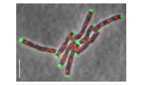
The data (courtesy of LMIC, EPFL, Lausanne, Switzerland) consist of several time-lapse microscopy videos showing the growth of M. smegmatis colonies. Images are composed of a phase contrast and a fluorescence channel reporting cellular division. In approximately the first 3/4 of the frames of each videos, the medial axis of the bacterias have been annotated with a custom software.

Ambiguity in single frame segmentation

The main issue with this data is that the detection relies mainly on the temporal data since on a given frame it is not obvious to the human eye where the boundaries of the cells are since cells are often cluttered.

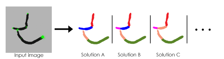
Here a simple input frame with fews cells can lead to multiple hypothesis on the number and placement of cells in the frame. This shows how there is ambiguity on individual cells detection even in a few cell setup. Later in the time-lapse there can be thousands of cells at once. Therefore, because of the in-frame ambiguity, we cannot simply segment each frame and then track between frames.

From that example one can intuit that some solutions are more likely than others, also by using the data from the previous and next frame we may have more insight on the most probable solution. For that matter we used a graphical model to make use of all of the data available in order to solve the detection and tracking.

---

Graphical models for joint Segmentation and tracking

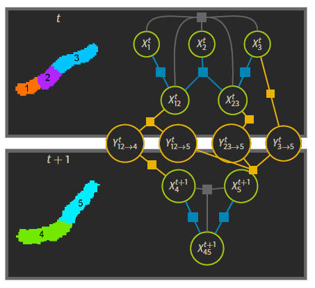
Schiegg et al. propose a model based on factor graphs to represent the multiple detection hypothesis and jointly tracking and segmenting on whole videos at once (Schiegg et al., 2014). To put it in a nutshell, given that we provide a set of detection candidates and transition candidates , along with associated probabilities , this method uses a graph representation to compute the most likely candidates for detections and transitions within some constraints .

• detection candidates are potential cells (for instance the region labeled 1 in the figure, or the union of 2 and 3 labeled 23)
• transition candidates represent how these candidates would transition from one frame to the next. Here one could expect 12 (at frame t)to transition into 4 (at frame t+1)
• constraints are what makes the solution physically sound, no cell candidates can overlap (cell candidate 12 could not co-exist with 23), cells should not appear and disappear in the middle of the video etc…

For each of the detection candidates and transition candidates we can provide an associated probability, this is provided by a simple classifier that uses as input some cell data (shape, length etc..) to infer its likelihood of being a cell or transition regardless of context. For instance a one pixel cell would have a very low probability and a transition implying that a cell would travel from one end of the image to the other in a single frame is also rated with a low probability.

To explain the technical functioning of a graphical model would take another presentation, for this time we will focus on how to generate these segmentation proposals. Also this part of the graphical inference model had already been implemented by C. Haubold (Haubold, 2017).

Graphical model model limitation

From the previous example we can expect the graph to grow exponentially as the number cell proposal augments. Thus it is important to generate a set of segmentation proposals that is wide enough to contain the ground truth but small enough not to make the complexity explode.

Previous approach

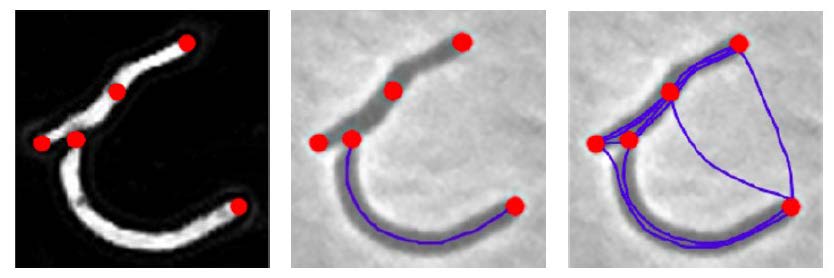
BactImAS (Mekterović et al., 2014) offers a semi-automated solution to the tracking problem where the user must manually define initial cells, division events, and maybe correct the model’s prediction in between. To detect cells BactImAS relies on edge detection, thresholds and skeletonization. In her PhD thesis (Uhlmann, 2017), Virginie Uhlman introduces splines to further automate the process. From the detected cell tips a set of shortest viable path in between are generated as cell proposals. The issue of the exploding graph complexity remains because of the high number of proposals.

---

Exploring candidates generation through deep learning

The aim of my internship project was to explore the generation of cell candidates using deep learning methods. The idea being that a number of cell proposal could be ruled out by their improbable shape, thus adding a learning component (opposed to doing only image processing) to the process could improve the proposals.

First approach : U-net for pixel class prediction

Graphical models provide a way to solve for the tracking and segmentation problem simultaneously on the entire video. However, it relies on cell candidates generated for each frame. Since we want the true segmentation to be within the set of candidates, we perform over-segmentation (i.e. we segment too much) to ensure that we obtain more false positives that false negatives (for that we can rule out false positives with the graphical model). Deep neural networks can be used to generate such segmentation proposals in a robust and generalisable way. For instance, (Falk et al., 2019) propose a deep learning method for detecting instances of cells in images relying on pixel-wise classification. For that matter we used a U-Net architecture.

What is a U-net ?

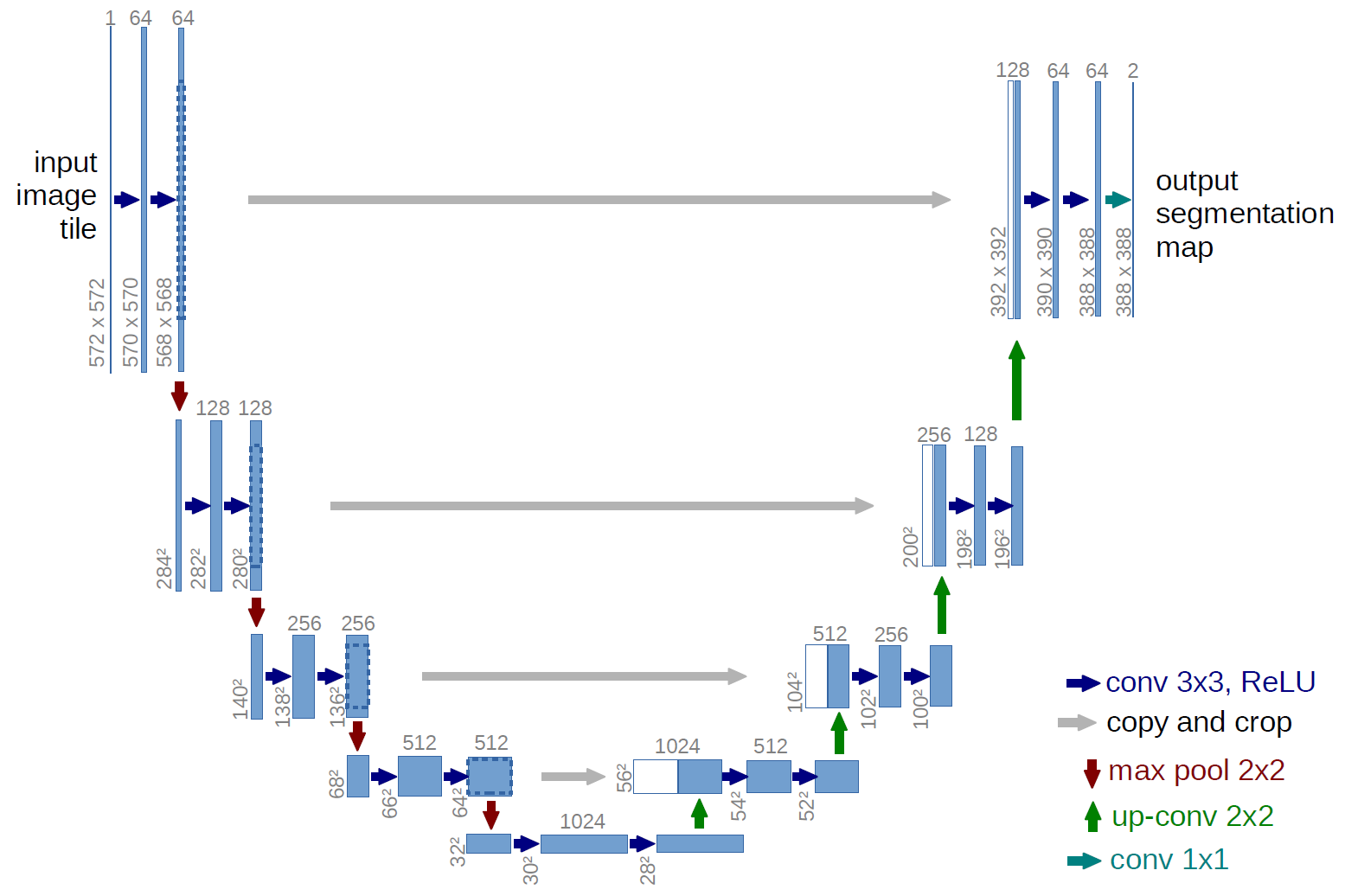
U-net is a convolutional neural network first introduced by (Ronneberger et al., 2015) for biomedical image segmentation. It aims at providing fine pixel classification with low and high scale awareness of the neighboring pixels. The network is composed of a contracting path that decreases the image size through convolution and pooling while increasing the number of channels, and an expansive path that increases the image size through convolution and up-sampling while decreasing the number of channels. The output image scale is therefore the same as the input. Skip paths are also added to link layers within levels, so that the information capturing fine details can be forwarded to the end of the network without traversing the contracting path.

Weighted soft-max cross-entropy loss

We use a Cross entropy loss with soft-max as it is commonly used for classification (Bishop, 2006) and can be written as

\[l(I) := - \sum_{x\in I}w(x) \log \frac{ \exp \left( \hat{y}_{y(x)}(x) \right) }{ \sum_{k=0}^K\exp \left( \hat{y}_{k}(x) \right) },\]

with \(x\) a pixel in the image domain \(I\), \(\hat{y}_k:I\rightarrow\mathbb{R}\) the predicted score for class \(k\), \(K\) the number of classes, and \(y:I\rightarrow\{0,\dots,K\}\) the ground truth segmentation. Thus, \(\hat{y}_{y(x)}(x)\) corresponds to the predicted score for ground-truth class \(y(x)\) at position \(x\). The \(w(x)\) is a per-pixel weighting term used to handle class imbalance and instance separation, and is defined as

\[w:=w_\mathrm{bal} +w_\mathrm{sep}\]

Learning instance segmentation

To learn how to segment instances, labels of different instances must be separated by at least one pixel of background, ensuring that each instance is one single connected component. In order for this gap to be predicted correctly by the network, a weighting term \(w_\mathrm{sep}\) is applied on the loss to further penalize errors in boundary areas as

\[w_\mathrm{sep}(x) := \exp \left( -\frac{(d_1(x)+d_2(x)}{2\sigma^2}\right),\]

with \(d_1\) and \(d_2\) the distances to the two nearest instances. This weight therefore increases at locations where two cells are close together, enforcing a separation. The next figure shows an illustration of \(w_\mathrm{sep}(x)\) over an image.

Pixel class prediction

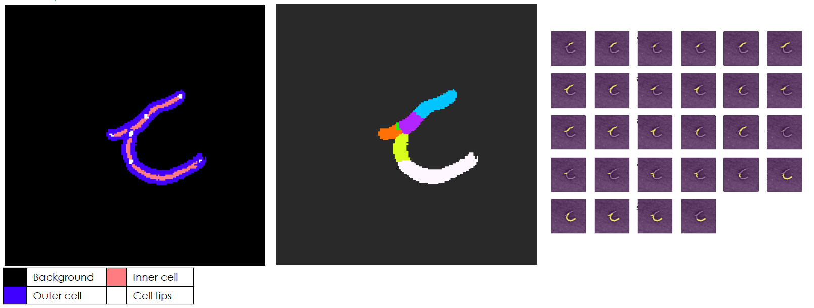
Our first objective is to distinguish cells from background, thus we use a background class and a cell class. However individual cells need to be spatially separated by a gap in order to distinguish different entities, hence we introduce an inner cell and outer cell class in order to have separate cell cores between and also not to confuse the classifier by labeling the outer cells as background. Since the cell tips will be a useful information to separate individual cells afterwards we also introduce a cell tip class.

Once the U-net is trained, the network outputs probability maps for each class.

Candidates generation

From output of the network we need to produce a set of cell candidates. We devised a method of over-segmentation to get a set of cell parts that could be assembled to make cell candidates. Basically, from the separated inner cells, we run a watershed algorithm to propagate labels on the cells. We get the results shown below on a sample image. From the over-segmentation output we can build a set of cell proposals. We build proposals from the cell segments by proposing every segment and every union of touching segments (within a set limit amount, so that cells aren’t too big).

Results

This pixel wise classification approach provided decent results, however the candidates generation part relies heavily on manually chosen hyper-parameters. Also this methods tends to generate quite a lot of very small cell proposals. These numerous false positive make the graphical model complexity explode. Any attempt at choosing a set of hyper-parameters to reduce the number of false positives dramatically increase the number of false negatives, meaning that the graphical model cannot be set up.

---

Instance segmentation with pixel embedding

In the first approach the instance segmentation (differentiating one cells from its neighbor) is done by the proxy of per pixel classification. What if we could directly optimize for instance segmentation within the convolutional network and thus minimize the handcrafting of the cell proposal method ?

We thus focus on a framework in which the instance segmentation problem becomes a pixel clustering problem in a new feature space (De Brabandere et al., 2017). This approach allows predicting instance segmentation with no prior on the number of elements in the image. In constrast to other popular instance segmentation methods like Mask R-CNN (He et al., 2017), it does not rely on region proposal followed by classification. Instead of doing pixel classification with a softmax loss, which would limit the number of instances, we can detect any number of instances in an image can be captured. Indeed, when predicting instances as one class for each instance, the number of instances is limited by the size of the output vector, i.e. the number of classes. Also (Payer et al., 2018) extend this idea by considering a tracking component to the problem, adding recurrent components in the network and using a new similarity measure in the feature space.

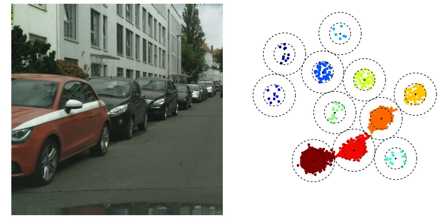
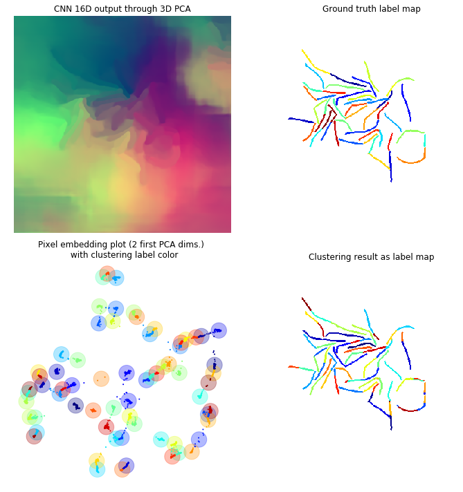
In this framework each pixel is attributed a N dimensional vector, so that every pixel from a same cell has a “similar” vector and pixels from different cells have “non-similar” vectors (the similarity measure may depend on the method used). If N=3 you can consider these vectors to be RGB colors, the objective being so that each individual cell is colored uniformly, but different cells have different colors. Through the different figures we project our N dimensional vectors to a 3D space with a PCA so that we can display these vectors as colors. Using the first two dimensions of the PCA we can plot these pixels as points within this 2D space to better visualize the clustering.

Semantic InstanceSegmentation with a Discriminative Loss Function

discriminative loss

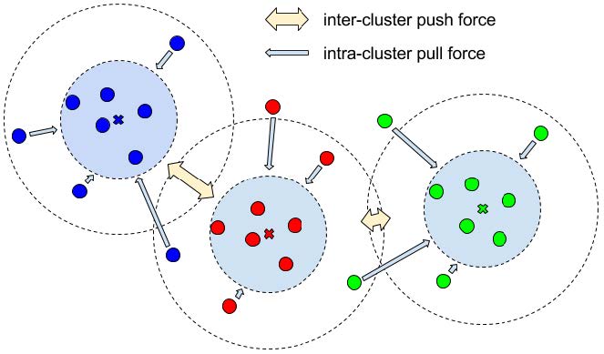
To learn the clustering, we rely on a discriminative loss composed of three key parts (De Brabandere et al., 2017). During learning we use as input the image along with ground truth instance labels.

• Variance term: is an intra-cluster pull force moving embeddings toward the mean of each label cluster. A margin is set for the variance, which corresponds to the inner circle in the next figure. This margin defines how tightly packed clusters should be.
• Distance term: an inter-cluster push force drawing the mean of embeddings of different instances further apart from each other. A margin is set for the distance, corresponding to the outer circle in the next figure. This margin defines how far from each other clusters should be.
• Regularization term: it is a pull force drawing clusters closer to the origin of the embedding space to avoid values blowing up.

These three part as summed as the loss function and minimized during the learning phase.

Clustering

For that matter, we used the agglomerative clustering available in sklearn (Pedregosa et al., 2011). This method starts by initializing each pixel as a cluster. Clusters are then merged together in a tree-like manner. The merging stops when a distance threshold is met, that is when the distance between all clusters is more than the threshold. This is relatable to the design of the discriminative loss since it enforces a minimal distance between different instances. Also this method does not rely on a prior knowledge of the number of clusters.

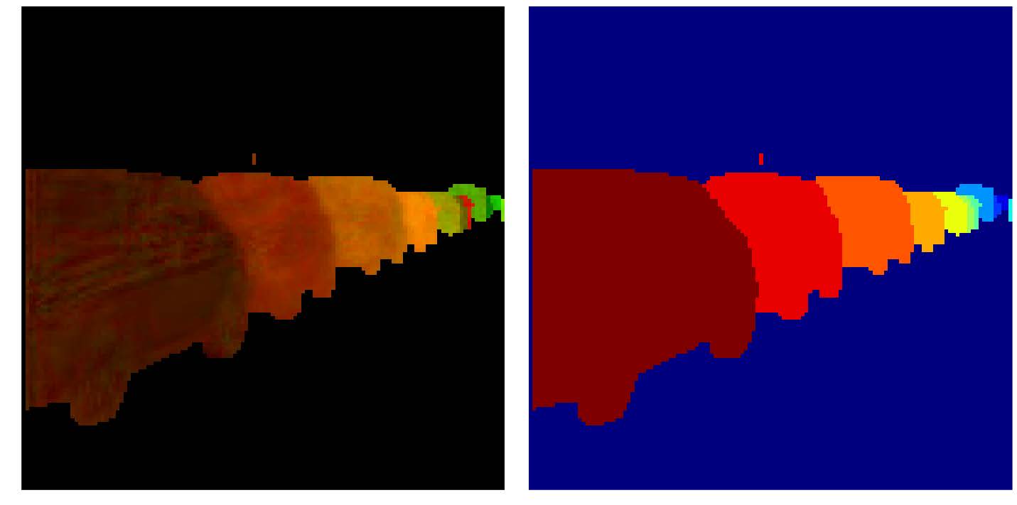
Results

Here is the results on a few sample frames. From the second more cluttered frame we observe that this method scales decently to a high number of cells. One improvement might be to add a filter on the smallest size a cluster can be to avoid 1 pixel clusters being proposed as cells.

---

Other approaches and perspectives

We tried implementing a Cosine embedding loss (Payer et al., 2018) as a replacement for the discriminative loss function. This yielded similar results but is not as straightforward to cluster as instead of using any N dimensional vector, the pixels are embedded in a N dimensional sphere. Meaning that the similarity function for clustering is not longer a simple euclidean distance but rather a cosine similarity. Also (Payer et al., 2018) proposes to compute the loss over several frame and ensure that cells have a consistent embedding cluster through time, thus learning the tracking part along the instance segmentation part. Due to time constraints I did not manage to properly test this promising method.

Another idea would be to expand this embedding time consistency to cell divisions, for instance we could devise a loss so that, once projected in a set of specified dimension parent cells would be similar, but remains separate in the other dimensions. If functioning properly this method would negate the need of the graphical model as it solves for tracking, instance segmentation and cell divisions at once.

---

Conclusion

From the different convolutional network methods I used I managed to produce strong sets of cell proposals. However due to time constraints and technical limitation of the graphical model, I did not manage to properly use these cell proposals to train the latter. Meanwhile this project gave me a great insight on the functioning and building on convolutional networks.

Throughout this project, the graphical model was a motivation for our model design choices. A U-net architecture provides an instance segmentation that is not satisfactory as it has extensive post-processing that is specific to the dataset. As we aim for generalizable solution we also explored instance segmentation oriented networks and losses (e.g. discriminative or cosine embedding loss). These offer a more straightforward optimization process to obtain cell candidates for the graphical model. Moreover, the clustering process offers better control on the roughness or finesse of the segmentation candidates.

Unfortunately, the ground truth matching part which is necessary to train the graphical model, proved to be a roadblock when using our first instance predictions obtained using U-net on a pixel classification task. We sadly did not have time to test ground piping our discriminative network results into the graphical model.

---

Acknowledgments

To the French Embassy in London for funding this internship, to EMBL for making it possible, to José for his technical help, And mostly, warm and sincere thanks to the whole Uhlmann Lab : Virginie, Soham, Yoann, Johannes, James and Maria.

---

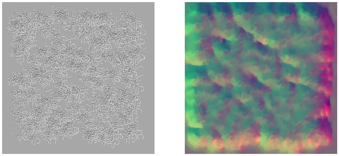
Bonus: Making some abstract “art” with it

As i noticed the network trained on the discriminative loss function outputted some pretty colors I tried to feed it a synthetic image over-packed with cells. This is the result, it makes for a great (but maybe too colorful) wallpaper.

---

References

1. Santi, I., Dhar, N., Bousbaine, D., Wakamoto, Y., & McKinney, J. D. (2013). Single-cell dynamics of the chromosome replication and cell division cycles in mycobacteria. Nature Communications, 4, 2470 EP -. https://doi.org/10.1038/ncomms3470
2. Santi, I., & McKinney, J. D. (2015). Chromosome Organization and Replisome Dynamics in Mycobacterium smegmatis. MBio, 6(1). https://doi.org/10.1128/mBio.01999-14
3. Ginda, K., Santi, I., Bousbaine, D., Zakrzewska-Czerwińska, J., Jakimowicz, D., & McKinney, J. (2017). The studies of ParA and ParB dynamics reveal asymmetry of chromosome segregation in mycobacteria. Molecular Microbiology, 105(3), 453–468.
4. Schiegg, M., Hanslovsky, P., Haubold, C., Koethe, U., Hufnagel, L., & Hamprecht, F. A. (2014). Graphical model for joint segmentation and tracking of multiple dividing cells. Bioinformatics, 31(6), 948–956.
5. Haubold, C. (2017). Scalable Inference for Multi-target Tracking of Proliferating Cells [PhD thesis].
6. Mekterović, I., Mekterović, D., & others. (2014). BactImAS: a platform for processing and analysis of bacterial time-lapse microscopy movies. BMC Bioinformatics, 15(1), 251.
7. Uhlmann, V. S. (2017). Landmark active contours for bioimage analysis: A tale of points and curves [PhD thesis]. Ecole Polytechnique Fédérale de Lausanne.
8. Falk, T., Mai, D., Bensch, R., Çiçek, Ö., Abdulkadir, A., Marrakchi, Y., Böhm, A., Deubner, J., Jäckel, Z., Seiwald, K., Dovzhenko, A., Tietz, O., Dal Bosco, C., Walsh, S., Saltukoglu, D., Tay, T. L., Prinz, M., Palme, K., Simons, M., … Ronneberger, O. (2019). U-Net: deep learning for cell counting, detection, and morphometry. Nature Methods, 16(1), 67–70. https://doi.org/10.1038/s41592-018-0261-2
9. Ronneberger, O., Fischer, P., & Brox, T. (2015). U-Net: Convolutional Networks for Biomedical Image Segmentation. CoRR, abs/1505.04597. http://arxiv.org/abs/1505.04597
10. Bishop, C. M. (2006). Pattern Recognition and Machine Learning (Information Science and Statistics). Springer-Verlag.
11. De Brabandere, B., Neven, D., & Van Gool, L. (2017). Semantic instance segmentation with a discriminative loss function. ArXiv Preprint ArXiv:1708.02551.
12. He, K., Gkioxari, G., Dollár, P., & Girshick, R. (2017). Mask r-cnn. Proceedings of the IEEE International Conference on Computer Vision, 2961–2969.
13. Payer, C., Štern, D., Neff, T., Bischof, H., & Urschler, M. (2018). Instance segmentation and tracking with cosine embeddings and recurrent hourglass networks. International Conference on Medical Image Computing and Computer-Assisted Intervention, 3–11.
14. Pedregosa, F., Varoquaux, G., Gramfort, A., Michel, V., Thirion, B., Grisel, O., Blondel, M., Prettenhofer, P., Weiss, R., Dubourg, V., Vanderplas, J., Passos, A., Cournapeau, D., Brucher, M., Perrot, M., & Duchesnay, E. (2011). Scikit-learn: Machine Learning in Python. Journal of Machine Learning Research, 12, 2825–2830.

---